Research — Digital payment pressure and bank net fee margins

Findings, step by step

From a pooled association to what it can and cannot claim

Six steps, each with the chart behind it. Scroll to read them, or present them one annotation at a time. Every chart links to the table rows it is drawn from.

The measure

Digital payments grew everywhere, from very different starting points

Mobile and internet banking transactions, measured as a share of GDP, rose in all three markets between 2014 and 2022: Indonesia from 111% to 268% and Malaysia from 366% to 719%, while Thailand more than quadrupled, from 124% to 532%.

The indicator counts transactions processed by banks themselves, not activity on non-bank FinTech platforms.

Numbers: the Data section

Mobile and internet banking transactions, % of GDP1 / 6

2014 and 2022 values for each country; the years in between are not drawn.

Across countries

Across countries, more digital intensity goes with lower fee margins

Averaged over the sample, Indonesian banks earn a net fee margin of 2.2% of assets at a digital intensity of 164% of GDP. Thailand (1.2% at 271%) and Malaysia (1.2% at 540%) are more digital and earn about one percentage point less.

Three countries make three points. This compares markets; it does not show change within any one of them.

Numbers: the robustness paragraph and the Data table

Country averages, 2014–20222 / 6

Each dot is one country's sample average. Labels give the number of bank-year observations.

The pooled model

The log model finds a negative, significant pooled association

With bank and year fixed effects and bank-clustered standard errors, the log baseline estimates −0.0102 (SE 0.0051, p = 0.048). In economic terms, doubling digital intensity goes with a net fee margin about 0.71 percentage points of assets lower, roughly 39% of the 1.81% sample mean.

The three linear specifications point the same way, but only the first reaches even marginal significance.

Numbers: the Results table

t-statistic by specification3 / 6

Each dot is a t-statistic: the published coefficient divided by its bank-clustered standard error. The scaled and log models use different units, so t is the comparable quantity. Dashed lines mark |t| = 1.645 (10%) and 1.96 (5%).

Where it comes from

Split the association, and it sits between countries

A Mundlak decomposition separates two sources of variation. The between-country coefficient, −0.0124, has the same sign and size as the pooled estimate, although with three countries it is imprecise (p = 0.48). The within-country coefficient, −0.0049 (p = 0.53), is less than half the pooled estimate and far from significant.

The pooled result mostly reflects differences between countries, not change within each country over time.

Numbers: the Robustness table

The pooled estimate, split into between and within4 / 6

Dots are estimates and bars are 95% intervals (estimate ± 1.96 × SE). Every row uses the log specification.

Country by country

Country by country, the sign is not the same

Estimated separately, with bank effects but no year effects, Indonesia is −0.0014 with a wide interval and Malaysia +0.0055, while Thailand is +0.0017, weakly positive. Thailand is also the market whose virtual-bank framework is led by incumbents, which fits a contestable-markets reading.

Few clusters: 9 Malaysian and 7 Thai banks.

Numbers: the country-subsample row and the limitations

Country subsamples, log specification5 / 6

Bank effects, no year effects, because a single-country model would absorb a country-year regressor into the year effects. Bars are 95% intervals.

What it can claim

What the evidence supports, and what it does not

Statistical significance is not economic importance, and neither is causality: the regressor varies only at the country-year level, about 27 distinct values. The next design would test a policy event, such as Malaysia's digital-bank licences (2020) or Thailand's virtual-bank framework (2024), with an event-study design and inference suited to few clusters.

Numbers: the Robustness, Hypotheses and Limitations rows

Claim ledger6 / 6

Each line restates a result from this page, with its estimate.

Step {n} Step {s} of {n} · note {c} of {m} Link copied: {h} Could not copy. The link is {u} Numbers behind step {n} Indonesia Malaysia Thailand Slope chart: mobile and internet banking transactions as a share of GDP in 2014 and 2022 for Indonesia, Malaysia and Thailand. {v}% of GDP Banks' own transactions only Scatter of country averages: Indonesia 2.2% net fee margin at 164% of GDP, Thailand 1.2% at 271%, Malaysia 1.2% at 540%. Average digital intensity, % of GDP Average net fee margin, % of assets {n} bank-years ≈ 1.0 pp lower 3 countries = 3 points {d}% of GDP · margin {m}% · {n} bank-years Dot plot of t-statistics for six specifications; the log baseline and the squared-term model pass |t| = 1.96. t = coefficient ÷ standard error LINEAR LOG Scaled measure + financial controls Full controls Log baseline Size interaction Squared log term p < 0.05 p < 0.10 not significant doubling ≈ −0.71 pp Interval plot: pooled estimates near −0.010, between-country −0.0124, within-country −0.0049 with an interval crossing zero. Coefficient on log digital intensity Pooled · clustered SE Pooled · Driscoll–Kraay Between countries Within countries Within-only FE same size less than half, p = 0.53 Interval plot by country: Indonesia −0.0014, Malaysia +0.0055, Thailand +0.0017. {n} obs incumbent-led virtual banks 9 Malaysian, 7 Thai banks {c} · 95% [{lo}, {hi}] · p {p} Supported by the data Not supported, or not claimed Next design A negative pooled association in the log model −0.0102, p = 0.048; Driscoll–Kraay p = 0.004 It shows in fees, not in lending Net-interest-margin placebo 0.0041, p = 0.45 Larger and negative with a one-year lag −0.0159, p = 0.062 A within-country effect −0.0049, p = 0.53 Larger banks are more resilient (H2) Interaction −0.0039, not significant A U-shaped recovery (H3) Squared term −0.0020, not significant A causal effect The regressor varies by country-year: about 27 values Event study on staggered licensing reforms Malaysia's digital-bank licences (2020), Thailand's virtual-bank framework (2024); wild-cluster bootstrap for few clusters

Question

Why the direction of the relationship is not obvious

Is digital payment pressure associated with bank net fee margins in Indonesia, Malaysia, and Thailand?

The question grew out of my Business Analytics Tableau project (December 2025). The study does not assume that digital payments help or hurt banks. Digitalisation can affect fee income through several channels at once, and they push in different directions:

Channel 1

Transaction and service expansion

Digital channels lower friction, increase usage, and can support new payment or merchant services.

Channel 2

Competitive pressure

FinTech firms, payment networks, and digital-first competitors may compress prices or reallocate payment-related revenue.

Channel 3

Customer relationships and cross-selling

Frequent digital engagement and transaction data can create opportunities in deposits, lending, insurance, or wealth management.

Channel 4

Institutional and market differences

Payment infrastructure, regulation, financial inclusion, and bank business models differ substantially across countries.

Two competing hypotheses, and two refinements

Hypothesis	Theory	Prediction	Result
H1a Substitution	Contestable markets (Baumol, 1982); liquidity adjustment costs (Verdier, 2024)	β₁ < 0	Consistent: negative and significant at 5% in the pooled log model
H1b Complementarity	Delegated monitoring (Diamond, 1984); bank–FinTech coexistence (Thakor, 2020); API and B2B alliances (Brandl and Hornuf, 2020)	β₁ > 0	Not supported
H2 Scale heterogeneity	Scale economies in technology (Berger, 2003)	Larger banks more resilient	Not supported: interaction −0.003930 (n.s.)
H3 Non-linear transition	Substitution first, complementarity as markets mature	U-shape, β₂ > 0	Not supported: squared term −0.001988 (n.s.)

H1a and H1b need not be mutually exclusive: competitive pressure may dominate early, while intermediation and platform channels strengthen as infrastructure matures, which is what H3 tests.

Because these channels can offset each other, a negative coefficient would not by itself show that digital payments reduce bank income. It could reflect market composition, country-specific institutions, or omitted factors that move together with both payment activity and bank outcomes.

Data

Two data levels joined into one panel

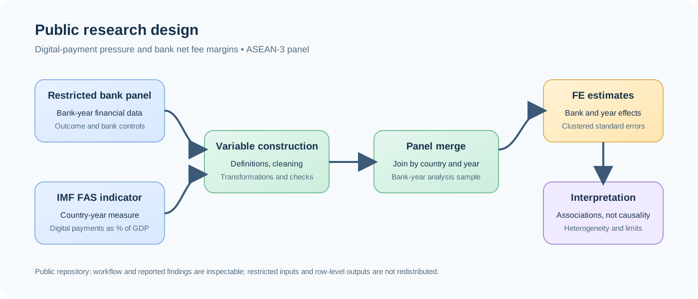
Bank-year financial variables form the outcome and controls; a country-year indicator measures digital payment activity.

Final analysis sample.
Item	Value
Countries	Indonesia, Malaysia, Thailand
Banks	39 publicly traded commercial banks and banking groups (including 3 Islamic and 5 digital-challenger banks)
Bank-year observations	344
Period	2014–2022
Study design	ASEAN-5 was originally planned; the selected indicator was not consistently available for the Philippines and Singapore
Observations by country	Indonesia 200 · Malaysia 81 · Thailand 63
Period rationale	2014: 4G roll-out and systematic payment monitoring begin; 2022: last year with complete audited reports for every bank.

Outcome and controls

Bank-year variables

Net_Fee_Margin — net fee and commission income relative to total assets, proxied by Compustat Global total non-interest income — the closest series available consistently across the three markets, which also contains trading and other non-interest revenue.
Size_USD — natural log of total assets converted into US dollars.
Capital_Adequacy_Proxy — equity-to-assets ratio (EQRAT in the thesis): book equity / total assets.
Credit_Risk — loan loss provisions / total assets.
Interest_Expense_Ratio — interest expense / total assets.
Deposit_Ratio — total deposits / total assets.

Explanatory measure

Country-year digital payment pressure

The explanatory variable comes from the IMF Financial Access Survey indicator IMF_FAS_FCMIBT, used with the unit PT_GDP: mobile and internet banking transactions as a percentage of GDP. It counts transactions processed by banks themselves, not by non-bank FinTech platforms. Between 2014 and 2022 it rose from 111% to 268% of GDP in Indonesia, from 366% to 719% in Malaysia and from 124% to 532% in Thailand. In the linear models one unit equals 10 percentage points of GDP (DPP_10pct_GDP); the refined models use ln(1 + DPP).

The indicator source is public; generated extraction files are not committed to the repository.
Availability, definitions, and reuse terms can change, so the workflow documents how the indicator was discovered and selected instead of treating it as a black box.

IMF Financial Access Survey

Method

Fixed effects, clustered inference, and explicit cleaning rules

The workflow separates panel preparation, indicator extraction, merging, estimation, and robustness checks, so each decision can be inspected on its own.

Flow diagram: restricted bank panel data and the public IMF Financial Access Survey indicator enter variable construction, then country-year merging, fixed-effects estimation, association results, and limitations. — Research design: restricted bank data and the public country-year indicator are constructed separately, then merged and estimated with bank and year fixed effects. The final stage records interpretation limits rather than causal claims.

Specification

NFM_it = β DPP_ct + γ′X_it + α_i + λ_t + ε_it

NFM is bank i's net fee margin in year t.
DPP is the digital-payment-pressure measure for country c in year t.
X is a vector of bank-level controls.
α is a bank fixed effect and λ is a year fixed effect, which absorb persistent bank differences and common time shocks.
The coefficient β is a conditional association inside the stated model, not an automatically causal effect.

Estimation choices

How the models were run

A complete-case sample is formed on the required outcome, explanatory variable, and controls so specifications are comparable.
Continuous variables are winsorised at the 1st and 99th percentiles within the analysis sample.
Standard errors are clustered at the bank level to account for dependence within bank histories. Driscoll–Kraay standard errors, robust to cross-sectional dependence, are reported alongside.
Country subsamples keep bank fixed effects and drop year effects, because a country-year explanatory variable would otherwise be absorbed in a single-country model.

Specifications tested

From baseline to robustness

Scaled digital-payment pressure (DPP_10pct_GDP).
Scaled pressure with additional financial controls, then a full-controls specification.
A logarithmic baseline (Log_Digital_Payment_Pressure).
A bank-size interaction (Digital_x_LargeBank).
A centred nonlinear specification with a squared log term.
Country-subsample estimates of the log specification.
Robustness: Driscoll–Kraay standard errors, a Mundlak between/within decomposition, excluding 2020, a net-interest-margin placebo, a one-year lag, and excluding Islamic and digital-challenger banks.

Results

Limited linear evidence, a significant logarithmic association

All models use the same 344 bank-year observations, so the specifications are directly comparable.

Digital-payment coefficient by specification. Bank-clustered standard errors. * p < 0.10, ** p < 0.05.
Specification	Coefficient	Std. error	Observations	R²	Interpretation
Main model, scaled measure	−0.000292*	(0.000177)	344	0.0065	Marginal Negative association with marginal statistical evidence.
Main model with controls	−0.000264	(0.000201)	344	0.0241	Not significant Negative sign but no statistical evidence.
Full controls model	−0.000208	(0.000333)	344	0.0739	Not significant Negative sign but no statistical evidence.
Log baseline model	−0.010171**	(0.005116)	344	0.0757	Significant Negative, statistically significant pooled association.
Size interaction model	−0.006507	(0.005227)	344	0.0796	Not significant Neither the Large Bank dummy nor its interaction with log pressure (−0.003930) is significant.
Nonlinear model	−0.010829**	(0.005432)	344	0.0766	Significant Negative linear term; the squared term (−0.001988) is not significant, so there is no U-shaped recovery.

How to read this table

The scaled and log models use different units, so the coefficient sizes are not comparable across rows; only the sign and significance are.
The pooled log association is statistically significant, but country subsamples are heterogeneous, and decomposition suggests the pooled result may substantially reflect differences between countries rather than a shared within-country mechanism.
Statistical significance is not the same as economic importance, and neither is the same as causality.
Economic size: in the log model, doubling digital-payment intensity is associated with a net fee margin about 0.71 percentage points of total assets lower (roughly 70 basis points), about 39% of the sample mean of 1.81%. Against the median (1.10%) the share is larger, so the percentage depends on the base.

Robustness and diagnostics

Test	Estimate	Interpretation
Driscoll–Kraay SE (Model 4)	−0.0102, SE 0.0035, p = 0.004 (bank-clustered p = 0.048)	Still significant when cross-sectional dependence is allowed
Driscoll–Kraay SE (Model 6 linear term)	−0.0108, SE 0.0032, p = 0.001 (bank-clustered p = 0.047)	Same
Mundlak decomposition: within	−0.0049, SE 0.0079, p = 0.53	No within-country association
Mundlak decomposition: between	−0.0124, SE 0.0175, p = 0.48	Same sign and size as the pooled estimate; imprecise with three countries
Within-only fixed effects	−0.0035, SE 0.0083, p = 0.67	Not significant
Country subsamples, no year effects	Indonesia −0.001420 (0.014970); Malaysia +0.005521 (0.005378); Thailand +0.001687* (0.000870)	Not uniform; Thailand weakly positive
Exclude 2020	Model 4 −0.008006 (0.004941), p = 0.106, n = 305	Similar size, less precise
Net interest margin placebo	0.004125 (0.005450), p = 0.45, n = 335	No effect on the lending margin: the pressure shows in the fee channel
One-year lag of regressor	−0.015901* (0.008475), p = 0.062, n = 305	Larger and negative; eases the reverse-causality concern
Exclude Islamic and digital-challenger banks	−0.004328 (0.002631), p = 0.101, n = 273, 31 banks	Smaller; part of the pooled size comes from this high-margin segment

The pooled negative association comes mainly from differences between countries — Indonesia averages a net fee margin of 0.022 at a digital intensity of 164% of GDP, Thailand 0.012 at 271%, Malaysia 0.012 at 540% — rather than from change within each country over time. That is the pattern contestable-markets theory predicts, because contestability is a property of market structure and entry conditions differ: Indonesia licenses e-money and peer-to-peer providers openly, Malaysia has issued digital-bank licences against mature incumbents, and Thailand's virtual-bank framework is led by incumbents — and it is in Thailand that the coefficient is weakly positive.

Limitations

What this study cannot claim

The results are conditional associations, not causal estimates. Eight constraints explain why.

Interpretation: a coefficient describes an association under a model, not an identified causal effect.
Data level and cluster counts: the explanatory measure varies only at the country-year level (about 27 distinct values across three countries and nine years), so the pooled estimate rests on few macro movements. Bank-level clustering (39 clusters) does not address cross-sectional correlation, which is why Driscoll–Kraay errors are also reported; country subsamples also have few clusters (9 Malaysian and 7 Thai banks).
Coverage: three countries are included, so the study should not be generalised to ASEAN-5 or all banking markets.
Omitted variables: regulation, payment infrastructure, macroeconomic conditions, and market concentration may affect both digital payments and fee margins.
Income aggregation: the outcome is total non-interest income over assets, so it cannot separate payment, card, merchant-service or wealth-management fees, and it also contains trading and other non-interest revenue.
Data access: the underlying bank panel cannot be redistributed, so the thesis regressions are inspectable but not publicly rerunnable.
What the pressure measure counts: the IMF indicator records banks' own mobile and internet banking transactions, not activity on non-bank FinTech platforms, so it measures the digital intensity banks operate in rather than direct FinTech competition.
Sample balance and timing: Indonesian banks supply 200 of the 344 observations (58%), weighting the pooled estimate toward that market, and reverse causality cannot be ruled out, although the lagged-regressor test reduces the concern.

Research agenda

What I would study next

The limitations above read as a research programme rather than a dead end. Four questions follow directly from them.

Identification

Separating within-country change from between-country structure

The decomposition is the starting point: the within-country coefficient is −0.0049 (p = 0.53) against a between-country −0.0124. The open question is what data would identify a within-country effect.

Heterogeneity

Which banks, and which business models

Size alone did not explain exposure: neither the Large Bank dummy nor its interaction was significant. Better measures of digital resilience, such as IT expenditure or the depth of platform and API partnerships, are the next step, alongside ownership and reliance on fee income.

Design

Designs that can identify a policy event

Staggered payment-licensing reforms are candidate events: Indonesia's e-money and peer-to-peer licensing, Malaysia's digital-bank licences (2020) and Thailand's virtual-bank framework (2024). A difference-in-differences or event-study design would first have to pass parallel-trends and treatment-definition tests, with inference suited to few clusters, such as a wild-cluster bootstrap.

Measurement

Finer revenue data than a single aggregate margin

Payments, cards, merchant services, and wealth management may not move together. Disaggregated fee income, and a payments measure closer to the bank than a country-year ratio, are the two changes most likely to sharpen the question.

This is the direction I am preparing to pursue in master's study. Nothing on this page claims it as a result of the completed project.

Reproducibility

Method transparency without data redistribution

The repository separates what can be rerun from what can only be inspected.

Component	Publicly reproducible?	Notes
Synthetic fixed-effects demonstration	Yes	Self-contained in `examples/run_example.py`, with a deterministic synthetic panel.
IMF FAS retrieval and indicator extraction	Partly	The source is public, but availability and terms can change; generated outputs are not committed.
Bank-panel construction and thesis regressions	No	Required WRDS-derived data and intermediate files are restricted and excluded.
Reported thesis findings	Inspectable only	The results are documented, but public files cannot regenerate them without the restricted inputs.

Run it yourself

Public demonstration in three commands

uv sync --group dev uv run python examples/run_example.py uv run pytest

The example uses deterministic synthetic data. It demonstrates the Python and linearmodels workflow; it is not evidence for the thesis.

Next steps

Where the research should go next

Disaggregate non-interest income into payments, cards, merchant services, and wealth management.
Broaden country coverage to restore the ASEAN-5 design.
Move towards identification: staggered payment-licensing reforms as quasi-experiments, difference-in-differences or event-study designs, an external instrument for digital adoption, and dynamic panel methods. (A one-year lag of the regressor is already reported in the thesis.)
Strengthen inference with few clusters: a wild-cluster bootstrap now, and country-level clustering once more countries are added. (Driscoll–Kraay standard errors are already reported in the thesis.)

Research process

Generative AI use

Tools used: ChatGPT, Claude, Google Gemini, and NotebookLM.

Brainstorming and identifying weaknesses in ideas.
Preliminary summaries of concepts and literature.
Planning the research schedule.
Grammar and spelling checks.
Assistance with regression and data-cleaning code.
Reference formatting.

All outputs were critically reviewed and independently verified.

Sources

Documentation behind this page

Everything below lives in the public repository. Restricted data, course submissions, and row-level outputs are deliberately excluded.

Public research report Design, results, limitations, and data-access boundaries.
Variable definitions Conceptual definitions without restricted observations.
Methodology appendix Workflow, specification, cleaning, and inference choices.
Main regression code Final specifications, retained for transparency. Robustness tables F3–F6 are reported in the thesis; their code is not yet in the public repository.
IMF Financial Access Survey Source of the country-year digital payment indicator.

The repository keeps bank identifiers, raw and derived datasets, submission drafts, feedback, and signatures out of the public surface. Check current WRDS, IMF, and university terms before redistributing any data or supporting material.